Simplicial homology

In mathematics, in the area of algebraic topology, simplicial homology is a theory with a finitary definition, and is probably the most tangible variant of homology theory.

Simplicial homology concerns topological spaces whose building blocks are n-simplexes, the n-dimensional analogs of triangles. By definition, such a space is homeomorphic to a simplicial complex (more precisely, the geometric realization of an abstract simplicial complex). Such a homeomorphism is referred to as a triangulation of the given space. Replacing n-simplexes by their continuous images in a given topological space gives singular homology. The simplicial homology of a simplicial complex is naturally isomorphic to the singular homology of its geometric realization. This implies, in particular, that the simplicial homology of a space does not depend on the triangulation chosen for the space.

It has been shown that all manifolds up to 3 dimensions allow for a triangulation. This, together with the fact that it is now possible to resolve the simplicial homology of a simplicial complex automatically and efficiently, make this theory feasible for application to real life situations, such as image analysis, medical imaging, and data analysis in general.

1 Definition
- 1.1 Example
2 Applications
3 See also
4 References
5 External links

Definition

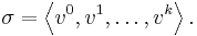
Let S be a simplicial complex. A simplicial k-chain is a formal sum of k-simplices

$\sum_{i=1}^N c_i \sigma^i \,$ , where $c_i \in \mathbb{Z}, \sigma^i \in S$ is the i-th k-simplex.

The group of k-chains on S, the free abelian group defined on the set of k-simplices in S, is denoted C_k.

Consider a basis element of C_k, a k-simplex,

$\sigma = \left \langle v^0 , v^1 , \dots ,v^k\right \rangle.$

The boundary operator

$\partial_k: C_k \rightarrow C_{k-1}$

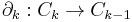
is a homomorphism defined by:

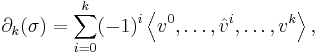
$\partial_k(\sigma)=\sum_{i=0}^k (-1)^i \left \langle v^0 , \dots , \hat{v}^i , \dots ,v^k\right \rangle ,$

where the simplex

$\left \langle v^0 , \dots , \hat{v}^i , \dots ,v^k\right \rangle$

is the i^th face of σ obtained by deleting its i^th vertex.

In C_k, elements of the subgroup

$Z_k = \ker \partial_k$

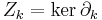
are referred to as cycles, and the subgroup

$B_k = \operatorname{im} \partial_{k%2B1}$

is said to consist of boundaries.

Direct computation shows that B_k lies in Z_k, that is, B_k ⊆ Z_k. The boundary of a boundary must be zero. In other words,

$(C_k, \partial_k)$

form a simplicial chain complex.

The k^th homology group H_k of S is defined to be the quotient

$H_k(S) = Z_k/B_k\, .$

A homology group H_k is not trivial if the complex at hand contains k-cycles which are not boundaries. This indicates that there are k-dimensional holes in the complex. For example consider the complex obtained by glueing two triangles (with no interior) along one edge, shown in the image. This is a triangulation of the figure eight. The edges of each triangle form a cycle. These two cycles are by construction not boundaries (there are no 2-chains). Therefore the figure has two "1-holes".

Holes can be of different dimensions. The rank of the homology groups, the numbers

$\beta_k = {\rm rank} (H_k(S))\,$

are referred to as the Betti numbers of the space S, and gives a measure of the number of k-dimensional holes in S.

Example

In order to compute the homology groups of the triangle, one should compute the different groups $\mathrm{ker}(\partial_0),\mathrm{Im}(\partial_1)$ etc. Here, by the definition of the boundary operator, we have $\partial_0([v_i]) = 0$ , therefore the kernel is:

$\mathrm{ker}(\partial_0) = C_0 = \{a_1[v_1] %2B a_2[v_2] %2B a_3[v_3] | a_1,a_2,a_3 \in \mathbb{Z}\} \cong \mathbb{Z} \oplus \mathbb{Z} \oplus \mathbb{Z}$

that is every 0-chain is in the kernel. Next, given a 1-chain $c_1 = b_1[v_1,v_2] %2B b_2[v_2,v_3] %2B b_3[v_3,v_1]$ there exists:

$\partial_1(c_1) = (b_3-b_1)[v_1] %2B (b_1-b_2)[v_2] %2B (b_2-b_3)[v_3]$

That is,

$\mathrm{Im}(\partial_1) = \{(b_3-b_1)[v_1] %2B (b_1-b_2)[v_2] %2B (b_2-b_3)[v_3] | b_1,b_2,b_3\in \mathbb{Z}\}$ ,

which means that a 0-chain $c_0 = a_1[v_1] %2B a_2[v_2] %2B a_3[v_3]$ is in the image of $\partial_1$ if and only if

$a_1 = b_3-b_1$

$a_2 = b_1-b_2$

$a_3 = b_2-b_3$ .

This implies that we have only two degrees of freedom for choosing $a_i$ , or in other words:

$\mathrm{Im}(\partial_1) \cong \mathbb{Z} \oplus \mathbb{Z}$

Now we can use the definition:

$H_0(S) \cong (\mathbb{Z} \oplus \mathbb{Z} \oplus \mathbb{Z})/ (\mathbb{Z} \oplus \mathbb{Z}) \cong \mathbb{Z}$

As for the other homology groups, computations are easier. $\partial_1(c_1) = 0$ if and only if $b_1=b_2=b_3$ , therefore

$\mathrm{ker}(\partial_1) = \{b[v_1,v_2] %2B b[v_2,v_3] %2B b[v_3,v_1] | b\in \mathbb{Z}\} \cong \mathbb{Z}.$

Now, since there are no 2-chains, the kernel and image of $\partial_2$ are trivial, that is $\mathrm{ker}(\partial_2) = \mathrm{Im}(\partial_2) = 0$ . This yields:

$H_1(S) = \mathrm{ker}(\partial_1) / \mathrm{Im}(\partial_2) = \mathrm{ker}(\partial_1) \cong \mathbb{Z}$

$H_2(S) = \mathrm{ker}(\partial_2) / \mathrm{Im}(\partial_3) \cong 0$

Applications

A standard scenario in many computer applications is a collection of points (measurements, dark pixels in a bit map, etc.) in which one wishes to find a topological feature. Homology can serve as a qualitative tool to search for such a feature, since it is readily computable from combinatorial data such as a simplicial complex. However, the data points have to first be triangulated, meaning one replaces the data with a simplicial complex approximation. Computation of persistent homology (Edelsbrunner et al.2002 Robins, 1999) involves analysis of homology at different resolutions, registering homology classes (holes) that persist as the resolution is changed. Such features can be used to detect structures of molecules, tumors in X-rays, and cluster structures in complex data. A MATLAB toolbox for computing persistent homology, Plex (Vin de Silva, Gunnar Carlsson), is available at this site.

References

Lee, J.M., Introduction to Topological Manifolds, Springer-Verlag, Graduate Texts in Mathematics, Vol. 202 (2000) ISBN 0-387-98759-2
Hatcher, A., Algebraic Topology, Cambridge University Press (2002) ISBN 0-521-79540-0. Detailed discussion of homology theories for simplicial complexes and manifolds, singular homology, etc.
Moise, E.E., Affine structures in 3-manifolds. V. The triangulation theorem and Hauptvermutung. Ann. Math. 96-114 (1952).

Simplicial homology

Contents

Definition

Example

Applications

See also

References

External links